Analyze Time-Series Data with Python and MongoDB Using PyMongoArrow and Pandas


Rate this tutorial


In today’s data-centric world, time-series data has become indispensable for driving key organizational decisions, trend analyses, and forecasts. This kind of data is everywhere — from stock markets and IoT sensors to user behavior analytics. But as these datasets grow in volume and complexity, so does the challenge of efficiently storing and analyzing them. Whether you’re an IoT developer or a data analyst dealing with time-sensitive information, MongoDB offers a robust ecosystem tailored to meet both your storage and analytics needs for complex time-series data.
MongoDB has built-in support to store time-series data in a special type of collection called a time-series collection. Time-series collections are different from the normal collections. Time-series collections use an underlying columnar storage format and store data in time-order with an automatically created clustered index. The columnar storage format provides the following benefits:
- Reduced complexity: The columnar format is tailored for time-series data, making it easier to manage and query.
- Query efficiency: MongoDB automatically creates an internal clustered index on the time field which improves query performance.
- Disk usage: This storage approach uses disk space more efficiently compared to traditional collections.
- I/O optimization: The read operations require fewer input/output operations, improving the overall system performance.
- Cache usage: The design allows for better utilization of the WiredTiger cache, further enhancing query performance.
In this tutorial, we will create a time-series collection and then store some time-series data into it. We will see how you can query it in MongoDB as well as how you can read that data into pandas DataFrame, run some analytics on it, and write the modified data back to MongoDB. This tutorial is meant to be a complete deep dive into working with time-series data in MongoDB.
We will be using the following tools/frameworks:
- MongoDB Atlas database, to store our time-series data. If you don’t already have an Atlas cluster created, go ahead and create one, set up a user, and add your connection IP address to your IP access list.
Note: Before running any code or installing any Python packages, we strongly recommend setting up a separate Python environment. This helps to isolate dependencies, manage packages, and avoid conflicts that may arise from different package versions. Creating an environment is an optional but highly recommended step.
At this point, we are assuming that you have an Atlas cluster created and ready to be used, and PyMongo and Jupyter Notebook installed. Let’s go ahead and launch Jupyter Notebook by running the following command in the terminal:

Once you have the Jupyter Notebook up and running, let’s go ahead and fetch the connection string of your MongoDB Atlas cluster and store that as an environment variable, which we will use later to connect to our database. After you have done that, let’s go ahead and connect to our Atlas cluster by running the following commands:
Next, we are going to create a new database and a collection in our cluster to store the time-series data. We will call this database “stock_data” and the collection “stocks”.
Here, we used the db.create_collection() method to create a time-series collection called “stock”. In the example above, “timeField”, “metaField”, and “granularity” are reserved fields (for more information on what these are, visit our documentation). The “timeField” option specifies the name of the field in your collection that will contain the date in each time-series document.
The “metaField” option specifies the name of the field in your collection that will contain the metadata in each time-series document.
Finally, the “granularity” option specifies how frequently data will be ingested in your time-series collection.
Now, let’s insert some stock-related information into our collection. We are interested in storing and analyzing the stock of a specific company called “XYZ” which trades its stock on “NASDAQ”.
We are storing some price metrics of this stock at an hourly interval and for each time interval, we are storing the following information:
- open: the opening price at which the stock traded when the market opened
- close: the final price at which the stock traded when the trading period ended
- high: the highest price at which the stock traded during the trading period
- low: the lowest price at which the stock traded during the trading period
- volume: the total number of shares traded during the trading period
Now that we have become an expert on stock trading and terminology (sarcasm), we will now insert some documents into our time-series collection. Here we have four sample documents. The data points are captured at an interval of one hour.
Now, let’s run a find query on our collection to retrieve data at a specific timestamp. Run this query in the Jupyter Notebook after the previous script.
//OUTPUT
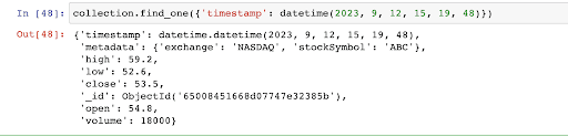
As you can see from the output, we were able to query our time-series collection and retrieve data points at a specific timestamp.
Similarly, you can run more powerful queries on your time-series collection by using the aggregation pipeline. For the scope of this tutorial, we won’t be covering that. But, if you want to learn more about it, here is where you can go:
Now, let’s see how you can move your time-series data into pandas DataFrame to run some analytics operations.
MongoDB has built a tool just for this purpose called PyMongoArrow. PyMongoArrow is a Python library that lets you move data in and out of MongoDB into other data formats such as pandas DataFrame, Numpy array, and Arrow Table.
Let’s quickly install PyMongoArrow using the pip command in your terminal. We are assuming that you already have pandas installed on your system. If not, you can use the pip command to install it too.
Now, let’s import all the necessary libraries. We are going to be using the same file or notebook (Jupyter Notebook) to run the codes below.
Now, we have read all of our stock data stored in the “stocks” collection into a pandas DataFrame ‘df’.
Let’s quickly print the value stored in the ‘df’ variable to verify it.
//OUTPUT
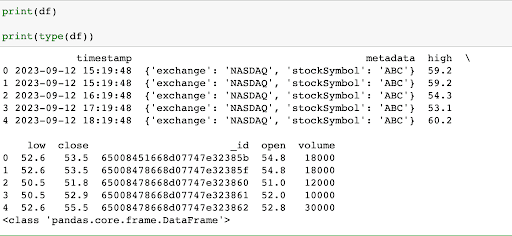
Hurray…congratulations! As you can see, we have successfully read our MongoDB data into pandas DataFrame.
Now, if you are a stock market trader, you would be interested in doing a lot of analysis on this data to get meaningful insights. But for this tutorial, we are just going to calculate the hourly percentage change in the closing prices of the stock. This will help us understand the daily price movements in terms of percentage gains or losses.
We will add a new column in our ‘df’ DataFrame called “daily_pct_change”.
//OUTPUT
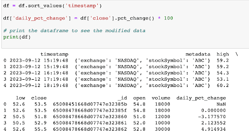
As you can see, we have successfully added a new column to our DataFrame.
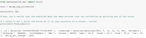
Now, we would like to persist the modified DataFrame data into a database so that we can run more analytics on it later. So, let’s write this data back to MongoDB using PyMongoArrow’s write function.
We will just create a new collection called “my_new_collection” in our database to write the modified DataFrame back into MongoDB, ensuring data persistence.
Congratulations on successfully completing this tutorial.
In this tutorial, we covered how to work with time-series data using MongoDB and Python. We learned how to store stock market data in a MongoDB time-series collection, and then how to perform simple analytics using a pandas DataFrame. We also explored how PyMongoArrow makes it easy to move data between MongoDB and pandas. Finally, we saved our analyzed data back into MongoDB. This guide provides a straightforward way to manage, analyze, and store time-series data. Great job if you’ve followed along — you’re now ready to handle time-series data in your own projects.
If you want to learn more about PyMongoArrow, check out some of these additional resources: